CE 319F LAB 5
5) MOMENTUM PRINCIPLE
5.1 OBJECTIVES
The primary objective of this laboratory is to learn about forces that
are needed to change the momentum of a flow. For this laboratory
all of the momentum changes are associated with convective acceleration.
For a water jet impinging on deflector vanes, the specific objectives are
-
Measure the force due to a momentum change for two types of jet deflectors.
-
Compare calculated and measured forces.
-
See that twice as much force is required when the momentum change increases
by a factor of two.
For air flow around a 90o bend, the specific objectives are
-
Observe that there is a high pressure on the outside of a bend and a low
pressure on the inside of a bend.
-
Understand that part of the support forces that are calculated using the
momentum equation comes from the resultant of the distributed pressures.
-
See that that the pressures and therefore the forces increase and decrease
as the flow rate increases or decreases since the magnitude of the acceleration
also increases or decreases.
5.2 BACKGROUND
5.2.1 Momentum Equations
The general momentum equation is
 |
(5.1) |
where  = force,
  = velocity,
  = unit outward vector on CS, which is the surface of the control volume
(C"). For steady flow with a constant
density, with discrete inflows and outflows, with essentially constant
velocities on each inflow and outflow cross section, and with the velocities
normal to the flow areas, the momentum equation can be written as
= unit outward vector on CS, which is the surface of the control volume
(C"). For steady flow with a constant
density, with discrete inflows and outflows, with essentially constant
velocities on each inflow and outflow cross section, and with the velocities
normal to the flow areas, the momentum equation can be written as
 |
(5.2) |
where Q = volumetric flow rate and = cross sectional average velocity vector with magnitude U.
5.2.2 Deflector Vanes
A jet flowing against a deflector vane is shown schematically in Fig. 5.1.
A vertical jet with velocity U1 strikes the vane and leaves
all around the vane with velocity U2. If the change in
elevation is negligible between cross sections 1 and 2 and if the shear
on the vane is negligible (as is the case for this experiment), then Bernoulli's
equation can be used to show that U1 = U2.
From continuity, Q1 = Q2. For the control volume
shown in Fig. 5.1, assuming that the weight of the fluid in the control
volume is negligible, the vertical (z) component of the momentum equation
(Eq. 5.2) gives
 |
(5.3) |
Fig. 5.1 - Schematic diagram of vertical jet and axisymmetric deflector
5.2.3 Bend
For the flow in a 90o bend with a constant cross sectional area
(Fig. 5.2), the convective acceleration or change in momentum comes from
changing the direction of the velocity, not the magnitude. Taking
the bend shown in Fig. 5.2 as the control volume, the x and z components
of Eq. 5.2 give
Rx = r(+U2)(+Q2)
= rU2Q2
Rz = r(-U1)(-Q1)
= rU1Q1 |
(5.3) |
where R is the resultant of the distributed positive pressure on the
outside of the bend and the distributed negative pressure on the inside
of the bend.
Fig. 5.2 - Schematic diagram of pressure distributions for air-flow
bend
5.3 LABORATORY APPARATUS
5.3.1 Jet
A photograph of the laboratory apparatus for the jet flow is shown in Fig.
5.3. The primary components are a vertical jet, two deflector vanes
which can be interchanged, and a lever arm for measuring the force of the
jet on the vane. One of the vanes is a flat, horizontal disk which
gives q = 0 (Fig. 5.1). The other one
is a hemispherical cup so that the flow leaving the vane is vertically
downward and q = -90o. The
apparatus is used on a hydraulic bench that provides the flow of water
and permits measurement of the flow rate.
5.3.2 Bend
An air flow can be established in a 90o bend with a rectangular
cross section. Tubes go from piezometer taps on the outside and inside
of the bend to the top of a multiple-tube, air-water manometer board.
The bottoms of all of the manometers are connected to the same constant
pressure reservoir. When the piezometer tap has a high pressure,
as on the outside of the bend, the water level in the manometer tube is
pushed down. A low pressure pulls the water level up from its equilibrium
position.
5.4 PROCEDURES
5.4.1 Jet
-
Install the flat vane (q = 0, Fig. 5.1).
-
Set the weight at the zero position on the weighing arm above the deflector
vane (Fig. 5.3), and adjust the spring (tare weight) so that the weighing
arm is horizontal, i.e., so that the all of the weights are balanced by
the spring.
-
Start the flow and adjust it to the desired flow rate.
-
Slide the weight along the weighing arm to bring it back to horizontal.
-
Measure the flow rate by weighing the amount of water (DW)
captured in the weighing tank in a measured time interval (Dt).
Then calculate the flow rate from Q = (DW/g)/Dt
= D"/Dt.
-
Calculate the force from Eq. 5.3 and compare it with the force obtained
from the moment equation for the weight.
-
Install the hemispherical vane (q = -90o).
Repeat steps 2-6. This force should be twice as large as for
the flat vane since the momentum change is twice as large. (From
Eq. 5.3, Fz = rQU for q
= 0, while Fz = 2rQU for q
= -90o.)
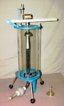
Fig. 5.3 - Laboratory apparatus for water jet
5.4.2 Bend
-
Adjust the reservoir and the water level in the reservoir on the left side
of the manometer board so that the water levels in the manometer tubes
are at 20 cm. Note that all of the water levels (including the tubes
open to the atmosphere) are the same.
-
Turn on the air flow and open the flow-control valve to obtain the maximum
possible flow rate.
-
Observe that the water levels in the manometer tubes connected to the outside
of the bend (i.e., the five tubes on the left side of the manometer board)
go down, indicating that the pressure has increased to a value above atmospheric
pressure, while the tubes connected to the inside of the bend indicate
a pressure that has decreased to be lower than atmospheric.
-
Note the manometer readings for the highest and lowest pressures.
-
Decrease the air flow.
-
Repeat steps 3 and 4 for the lower flow rate.
-
Note that the pressure changes are smaller for the lower flow rate.
Since the force (R) is the resultant of the distributed pressures, R also
decreases as the flow rate decreases.